November, 05, 2020

Computed Torque Control of a 3R Robot Arm Playing Ping Pong

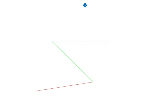
In this post, you will find the MATLAB and Simulink codes for equations of motions of a 3R (3 revolute joints) robot, Computed Torque Control of the 3R robot arm in joint and task spaces, and the 3R robot arm playing Ping Pong.

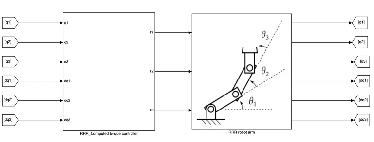
Suppose we have a 3R robot arm with 3 revolute joints pictured in the figure below:

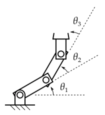
Fig. 1. A 3R (3 revolute joints) Serial Manipulator Robot

The following problems are going to deal with the simulations of the equations of motion of this robot using the Lagrange-Euler method, Computed Torque Control (CTC) of the 3R robot in joint and task spaces, and the 3R robot arm playing Ping Pong.

Problem 1.

Objective: Derive the equations of motion of the 3R serial manipulator robot using Lagrange-Euler method and simulating them in MATLAB and Simulink.

Note: Because it is a planar problem with all rotations about the z-axis, only the principle moment about the z-axis is relevant to derive the equations of motion for the robot.

Solution:

Please download the files at the end of this post and look at the RRR Dynamics folder. Note that you should have MATLAB and Simulink installed on your system to be able to run the codes.

The following shows the schematic of the dynamics of the robot in Simulink:

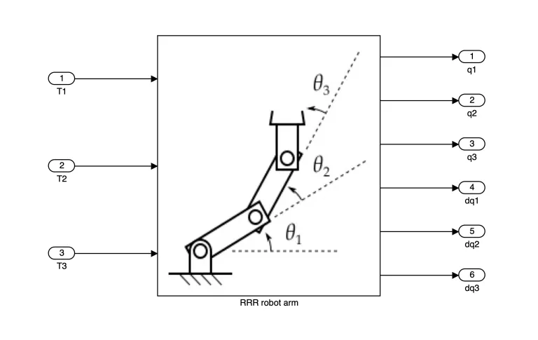
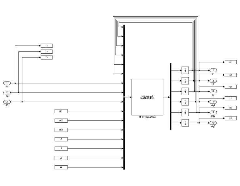
A 3R Serial Robot Manipulator Dynamics Implemented in Simulink

The “RRR_Dynamics” function used in the Simulink is as follows:

function dx = RRR_Dynamics(x)
% Joint positions
q1 = x(1);
q2 = x(2);
q3 = x(3);
% Joint velocities
dq1 = x(4);
dq2 = x(5);
dq3 = x(6);
% Joint Torques
T1 = x(7);
T2 = x(8);
T3 = x(9);
% Robot Parameters
m1 = x(10);
m2 = x(11);
m3 = x(12);
L1 = x(13);
L2 = x(14);
L3 = x(15);
W = x(16);
g0 = 9.81;
% Joint Position, Velocity and Torque Vectors
 q = [ q1;q2;q3];
dq = [dq1;dq2;dq3];
 T = [ T1;T2;T3];
 
 %%%%%%%%%%%%%%%%%%%%%%%%%%%%%%%%%%%%%%%%%%%%%%%%%%%%%%%%
 
 
robot_params =[];
robot_params(1) = m1 ;
robot_params(2) = m2 ;
robot_params(3) = m3 ;
robot_params(4) = L1;
robot_params(5) = L2;
robot_params(6) = L3;
robot_params(7) = W;
%%%%%%%%%%%%%%%%%%%%%%%%%%%%%%%%%%%%%%%%%%%%%%%%%
% Dynamics of planar 3-link robot arm
[M,C,G] = RRR_Dynamic_Matrices(q,dq,robot_params);
 
f  = [dq;         -inv(M)*(C*dq+G)];
G  = [zeros(3,3);  inv(M)];
dx = f+G*T;
end

And the “RRR_Dynamic_Matrices” function used in the above code (that contains the equations of motion of the 3R robot arm) is as follows:

function [M,C,G] = RRR_Dynamic_Matrices(q,dq,robot_params)
% This function derives the dynamic parameters of the Robot
m1 = robot_params(1);
m2 = robot_params(2);
m3 = robot_params(3);
L1 = robot_params(4);
L2 = robot_params(5);
L3 = robot_params(6);
W = robot_params(7);
g0 = 9.81;
%%%%%%%%%%%%%%%%%%%%%%%%%%%%%%%%%%
q1 = q(1);
q2 = q(2);
q3 = q(3);
dq1 = dq(1);
dq2 = dq(2);
dq3 = dq(3);
%%%%%%%%%%%%%%%%%%%%%%%%%%%%%%%%%%
%Mass Inertia Matrices
M(1,1) = (1/3).*L1.^2.*m1+L1.^2.*m2+(1/3).*L2.^2.*m2+L1.^2.*m3+L2.^2.*m3+(1/3).*...
  L3.^2.*m3+(1/12).*m1.*W.^2+(1/12).*m2.*W.^2+(1/12).*m3.*W.^2+L1.*L2.*...
  m2.*cos(q2)+2.*L1.*L2.*m3.*cos(q2)+L2.*L3.*m3.*cos(q3)+L1.*...
  L3.*m3.*cos(q2+q3);
M(1,2) = (1/3).*L2.^2.*m2+L2.^2.*m3+(1/3).*L3.^2.*m3+(...
  1/12).*m2.*W.^2+(1/12).*m3.*W.^2+(1/2).*L1.*L2.*m2.*cos(q2)+L1.*L2.*...
  m3.*cos(q2)+L2.*L3.*m3.*cos(q3)+(1/2).*L1.*L3.*m3.*cos(q2+...
  q3);
M(1,3) = (1/3).*L3.^2.*m3+(1/12).*m3.*W.^2+(1/2).*L2.*L3.*m3.*cos(q3)+...
  (1/2).*L1.*L3.*m3.*cos(q2+q3);
M(2,1) = M(1,2);
M(2,2) = (1/3).*L2.^2.*m2+L2.^2.*m3+(1/3).*L3.^2.*m3+(...
  1/12).*m2.*W.^2+(1/12).*m3.*W.^2+L2.*L3.*m3.*cos(q3);
M(2,3) =(1/3).*L3.^2.*...
  m3+(1/12).*m3.*W.^2+(1/2).*L2.*L3.*m3.*cos(q3) ;
M(3,1) = M(1,3);
M(3,2) = M(2,3);
M(3,3) = (1/3).*L3.^2.*m3+(1/12).*m3.*W.^2;
%%%%%%%%%%%%%%%%%%%%%%%%%%%%%%%%
%Ceriolis and Centrifugal Terms
C = zeros(3,3);
C1(1,1) = (-1).*dq2.*L1.*L2.*m2.*sin(q2)+(-2).*dq2.*L1.*L2.*m3.* ...
  sin(q2)+(-1).*dq3.*L2.*L3.*m3.*sin(q3)+(-1).*dq2.* ...
  L1.*L3.*m3.*sin(q2+q3)+(-1).*dq3.*L1.*L3.*m3.*sin(q2+ ...
  q3);
C1(1,2) = (-1).*dq1.*L1.*L2.*m2.*sin(q2)+(-1).*dq2.*L1.* ...
  L2.*m2.*sin(q2)+(-2).*dq1.*L1.*L2.*m3.*sin(q2)+(-2).* ...
  dq2.*L1.*L2.*m3.*sin(q2)+(-1).*dq3.*L2.*L3.*m3.*sin( ...
  q3)+(-1).*dq1.*L1.*L3.*m3.*sin(q2+q3)+(-1).* ...
  q2.*L1.*L3.*m3.*sin(q2+q3)+(-1).*dq3.*L1.*L3.*m3.* ...
  sin(q2+q3);
C1(1,3) = (-1).*dq1.*L2.*L3.*m3.*sin(q3)+(-1).* ...
  dq2.*L2.*L3.*m3.*sin(q3)+(-1).*dq3.*L2.*L3.*m3.*sin( ...
  q3)+(-1).*dq1.*L1.*L3.*m3.*sin(q2+q3)+(-1).* ...
  dq2.*L1.*L3.*m3.*sin(q2+q3)+(-1).*dq3.*L1.*L3.*m3.* ...
  sin(q2+q3);
C1(2,1) = (-1/2).*dq2.*L1.*L2.*m2.*sin(q2)+(-1).* ...
  dq2.*L1.*L2.*m3.*sin(q2)+(-1).*dq3.*L2.*L3.*m3.*sin( ...
  q3)+(-1/2).*dq2.*L1.*L3.*m3.*sin(q2+q3)+(-1/2).* ...
  dq3.*L1.*L3.*m3.*sin(q2+q3);
C1(2,2) = (-1/2).*dq1.*L1.*L2.* ...
  m2.*sin(q2)+(-1).*dq1.*L1.*L2.*m3.*sin(q2)+(-1).* ...
  dq3.*L2.*L3.*m3.*sin(q3)+(-1/2).*dq1.*L1.*L3.*m3.*sin( ...
  q2+q3);
C1(2,3) =(-1).*dq1.*L2.*L3.*m3.*sin(q3)+(-1).* ...
  dq2.*L2.*L3.*m3.*sin(q3)+(-1).*dq3.*L2.*L3.*m3.*sin( ...
  q3)+(-1/2).*dq1.*L1.*L3.*m3.*sin(q2+q3);
C1(3,1) = (-1/2).* ...
  dq3.*L2.*L3.*m3.*sin(q3)+(-1/2).*dq2.*L1.*L3.*m3.*sin( ...
  q2+q3)+(-1/2).*dq3.*L1.*L3.*m3.*sin(q2+q3);
C1(3,2) =(-1/2).* ...
  dq3.*L2.*L3.*m3.*sin(q3)+(-1/2).*dq1.*L1.*L3.*m3.*sin( ...
  q2+q3);
C1(3,3) =(-1/2).*dq1.*L2.*L3.*m3.*sin(q3)+(-1/2).* ...
  dq2.*L2.*L3.*m3.*sin(q3)+(-1/2).*dq1.*L1.*L3.*m3.*sin( ...
  q2+q3);
C2(1,1) = 0;
C2(1,2) = 0; 
C2(1,3) = 0;
C2(2,1) =(-1).*dq1.*L1.*L2.*m2.*sin(q2)+(-1/2).*dq2.*L1.* ...
  L2.*m2.*sin(q2)+(-2).*dq1.*L1.*L2.*m3.*sin(q2)+(-1).* ...
  dq2.*L1.*L2.*m3.*sin(q2)+(-1).*dq1.*L1.*L3.*m3.*sin( ...
  q2+q3)+(-1/2).*dq2.*L1.*L3.*m3.*sin(q2+q3)+(-1/2).* ...
  dq3.*L1.*L3.*m3.*sin(q2+q3);
C2(2,2) =(-1/2).*dq1.*L1.*L2.* ...
  m2.*sin(q2)+(-1).*dq1.*L1.*L2.*m3.*sin(q2)+(-1/2).* ...
  dq1.*L1.*L3.*m3.*sin(q2+q3);
C2(2,3) = (-1/2).*dq1.*L1.*L3.* ...
  m3.*sin(q2+q3);
C2(3,1) =(-1).*dq1.*L2.*L3.*m3.*sin(q3)+(-1).* ...
  dq2.*L2.*L3.*m3.*sin(q3)+(-1/2).*dq3.*L2.*L3.*m3.*sin( ...
  q3)+(-1).*dq1.*L1.*L3.*m3.*sin(q2+q3)+(-1/2).* ...
  dq2.*L1.*L3.*m3.*sin(q2+q3)+(-1/2).*dq3.*L1.*L3.* ...
  m3.*sin(q2+q3);
C2(3,2) =(-1).*dq1.*L2.*L3.*m3.*sin(q3)+(-1).* ...
  dq2.*L2.*L3.*m3.*sin(q3)+(-1/2).*dq3.*L2.*L3.*m3.*sin( ...
  q3)+(-1/2).*dq1.*L1.*L3.*m3.*sin(q2+q3);
C2(3,3) =(-1/2).* ...
  dq1.*L2.*L3.*m3.*sin(q3)+(-1/2).*dq2.*L2.*L3.*m3.*sin( ...
  q3)+(-1/2).*dq1.*L1.*L3.*m3.*sin(q2+q3);
C = C1 + C2;
%%%%%%%%%%%%%%%%%%%%%%%%%%%%%%%%%%%%%%%%%%%
% Gravity Terms
G = zeros(3,1);
G(1) = (1/2).*g0.*(L1.*(m1+2.*(m2+m3)).*cos(q1)+L2.*(m2+2.*m3).*cos(q1+ ...
  q2)+L3.*m3.*cos(q1+q2+q3));
G(2) = (1/2).*g0.*(L2.*(m2+2.*m3).* ...
  cos(q1+q2)+L3.*m3.*cos(q1+q2+q3));
G(3) = (1/2).*g0.*L3.*m3.* ...
  cos(q1+q2+q3);
end

Problem 2.

Objective: Defining a desired robot arm trajectory in joint space {qd,q̇d,q̈d} and implementing the torque control law to achieve the trajectory using the method of the Computed Torque Control law (see Chapter 4 Sections 5.1 and 5.2 of A Mathematical Introduction to Robot Manipulation by Murray, Li, and Sastry).

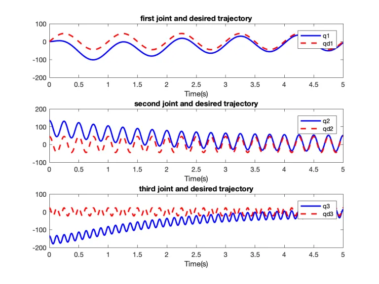
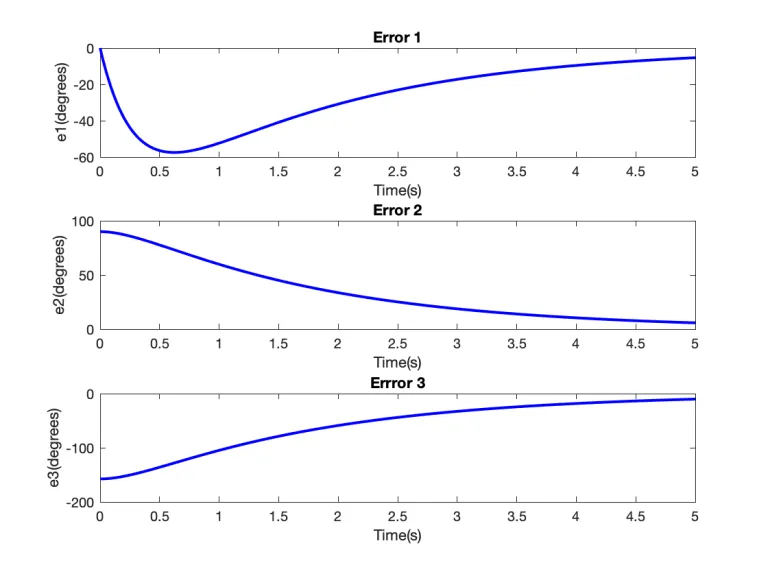
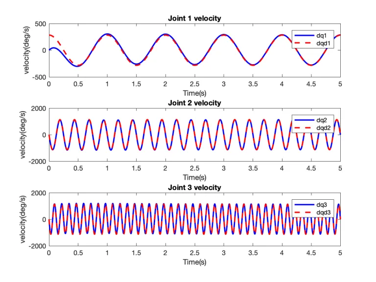
We want to show that even if the robot doesn’t start on the trajectory that it will converge to the desired trajectory.

Note: If you define the desired trajectory qd(t) analytically, then you can compute the first and second derivatives.

Solution:

Please download the files at the end of this post and look at the “RRR CTC Tracking Joint Space” folder. Note that you should have MATLAB and Simulink installed on your system to be able to run these codes.
The following shows the schematic of the Computed Torque Control of the 3R robot arm in joint space in Simulink:

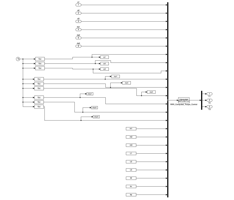
A 3R Serial Robot Manipulator with Computed Torque Control in Joint Space

The “RRR_computed_torque_control” function is as follows:

function T = RRR_CTC(x)
q1 = x(1);
q2 = x(2);
q3 = x(3);
dq1 = x(4);
dq2 = x(5);
dq3 = x(6);
qd1 = x(7);
qd2  = x(8);
qd3 = x(9);
dqd1 =x(10);
dqd2 = x(11);
dqd3 = x(12);
ddqd1 = x(13); 
ddqd2 = x(14);
ddqd3 = x(15);
m1 = x(16);
m2 = x(17);
m3 = x(18); 
L1 = x(19);
L2 = x(20);
L3 = x(21);
W = x(22);
kv = x(23);
kp = x(24);
%%%%%%%%%%%%%%%%%%%%%%%%%%%%%%%%%%%%%%%%%%%%%%%
params =[];
params(1) = m1;
params(2) = m2;
params(3) = m3; 
params(4) = L1;
params(5) = L2;
params(6) = L3;
params(7) = W;
%%%%%%%%%%%%%%%%%%%%%%%%%%%%%%%%%%%%%%%
% position, velocity and desired position vectors
q = [q1;q2;q3];
dq = [dq1;dq2;dq3];
qd = [qd1;qd2;qd3];
dqd = [dqd1;dqd2;dqd3];
ddqd = [ddqd1;ddqd2;ddqd3];
%%%%%%%%%%%%%%%%%%%%%%%%%%%%%%%%%%%%%%%%%%%5
% computed torque controller
[M,C,G] = RRR_Dynamic_Matrices(q,dq,params);
KV     =  kv*eye(3,3);
KP     =  kp*eye(3,3);
v       =  ddqd-KV*(dq-dqd)-KP*(q-qd);
T       =  M*v+C*dq+G;

The main code to run and get the outputs of the controller is as follows:

%the main program
clc
clear
% RRR Parameters
L1 = 2 ;
L2 = 2;
L3 = 2;
m1 = 0.1;
m2 = 0.1;
m3 = 0.1;
W = 0.01;
g = 9.81;
%%%%%%%%%%%%%%%%%%%%%%%%%%%%%%%%%%%%
%Controller
kv = 4;
kp = 2;
%%%%%%%%%%%%%%%%%%%%%%%%%%%%%%%%%%%%%%%%
% simulation parameters
T_f = 5; % simulation interval
AT = 1e-6; % absolute tolerance
RT = 1e-6; % relative tolerance
RF = 4; % Refine factor
%%%%%%%%%%%%%%%%%%%%%%%%%%%%%%%%%%%%%%%
% start simulation
q1 = [];
q2 =[];
q3 = [];
dq1 =[];
dq2 = [];
dq3 =[];
T1 = [];
T2 = [];
T3 = [];
sim('RRR_with_CTC')
%%%%%%%%%%%%%%%%%%%%%%%%%%%%%%%%%%%%%%%
% plot results
figure
subplot(3,1,1)
plot(tout,q1*180/pi,'b','linewidth',2)
hold on
plot(tout,qd1*180/pi,'r--','linewidth',2)
legend('q1','qd1')
xlabel('Time(s)')
title('first joint and desired trajectory')
subplot(3,1,2)
plot(tout,q2*180/pi,'b','linewidth',2)
hold on
plot(tout,qd2*180/pi,'r--','linewidth',2)
legend('q2','qd2')
xlabel('Time(s)')
title('second joint and desired trajectory')
subplot(3,1,3)
plot(tout,q3*180/pi,'b','linewidth',2)
hold on
plot(tout,qd3*180/pi,'r--','linewidth',2)
legend('q3','qd3')
xlabel('Time(s)')
title('third joint and desired trajectory')
figure
subplot(3,1,1)
plot(tout,T1,'b','linewidth',2)
xlabel('Time(s)')
ylabel('T1(Nm)')
title('Torque 1')
subplot(3,1,2)
plot(tout,T2,'b','linewidth',2)
xlabel('Time(s)')
ylabel('T2(Nm)')
title('Torque 2')
subplot(3,1,3)
plot(tout,T3,'b','linewidth',2)
xlabel('Time(s)')
ylabel('T3(Nm)')
title('Torque 3')
% errors
e1 = q1 - qd1;
e2 = q2 - qd2;
e3 = q3 - qd3;
figure
subplot(3,1,1)
plot(tout,e1*180/pi,'b','linewidth',2)
xlabel('Time(s)')
ylabel('e1(degrees)')
title('Error 1')
subplot(3,1,2)
plot(tout,e2*180/pi,'b','linewidth',2)
xlabel('Time(s)')
ylabel('e2(degrees)')
title('Error 2')
subplot(3,1,3)
plot(tout,e3*180/pi,'b','linewidth',2)
xlabel('Time(s)')
ylabel('e3(degrees)')
title('Errror 3')
figure
subplot(3,1,1)
plot(tout,dq1*180/pi,'b','linewidth',2)
hold on
plot(tout,dqd1*180/pi,'r--','linewidth',2)
legend('dq1','dqd1')
xlabel('Time(s)')
ylabel('velocity(deg/s)')
title('Joint 1 velocity')
subplot(3,1,2)
plot(tout,dq2*180/pi,'b','linewidth',2)
hold on
plot(tout,dqd2*180/pi,'r--','linewidth',2)
legend('dq2','dqd2')
xlabel('Time(s)')
ylabel('velocity(deg/s)')
title('Joint 2 velocity')
subplot(3,1,3)
plot(tout,dq3*180/pi,'b','linewidth',2)
hold on
plot(tout,dqd3*180/pi,'r--','linewidth',2)
legend('dq3','dqd3')
xlabel('Time(s)')
ylabel('velocity(deg/s)')
title('Joint 3 velocity')
figure
% Plot the links
for i = 1:length(q1)
  x0 = [0 0];
  x1 = [L1*cos(q1(i)) L1*sin(q1(i))];
  x2 = x1 + [L2*cos(q1(i)+q2(i)) L2*sin(q1(i)+q2(i))];
  x3 = x2 + [L3*cos(q1(i)+q2(i)+q3(i)) L3*sin(q1(i)+q2(i)+q3(i))];
 
  cla;
  hold on;
  plot([x0(1) x1(1)], [x0(2) x1(2)], 'r-');
  plot([x1(1) x2(1)], [x1(2) x2(2)], 'g-');
  plot([x2(1) x3(1)], [x2(2) x3(2)], 'b-');
  axis([-8 8 -8 8])
  drawnow
end

The desired joint trajectories are defined as follows:

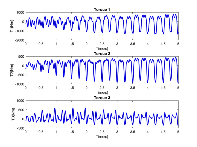
q_{d 1} = \frac{π}{4} s i n (2 π t) q_{d 2} = \frac{π}{4} s i n (8 π t) q_{d 3} = \frac{π}{8} s i n (16 π t)

By running the main code you will see the following outputs:

Computed Torque Control (CTC) of a 3R Robot Arm in Joint Space

Computed Torque Control (CTC) of a 3R Robot Arm in Joint Space – Joint Torques

Computed Torque Control (CTC) of a 3R Robot Arm in Joint Space – Errors

The Computed Torque Control (CTC) of a 3R Robot Arm in Joint Space – Joint Velocities

Problem 3.

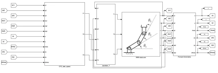
Objective: Deriving the form of the robot equation in task space (see Chapter 4 Section 5.4 of A Mathematical Introduction to Robot Manipulation by Murray, Li, and Sastry) and implementing the computed torques/forces control method to cause the robot to follow the desired trajectory.
For the next problem of juggling the ball, a good choice of the desired trajectory should probably be vertical motion with the end effector held flat.

Note: Even when we have converted the equations to the task space form of the robot equation, the “true system” still only accepts joint torques.

So, after computing the appropriate configuration space forces/torques using the method of computed torques, these need to be converted back into joint torques for the simulation. See the page following Lemma 4.11 in the book for a more thorough description.

Solution:

Please download the files at the end of this post and look at the “RRR CTC Task Space” folder. Note that you should have MATLAB and Simulink installed on your system to be able to run these codes.

The following shows the schematic of the Computed Torque Control of the 3R robot arm in task space in Simulink:

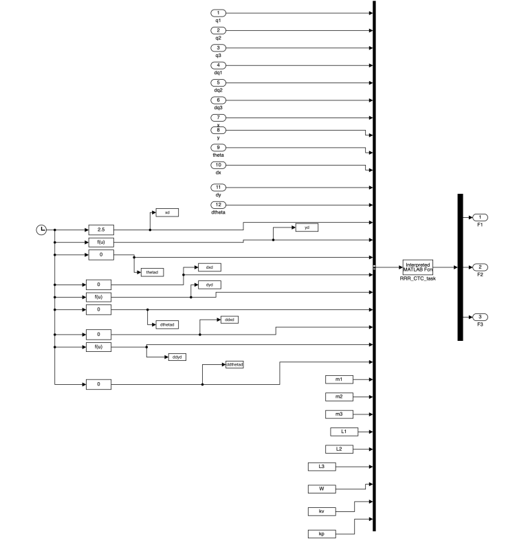
The schematic of the Computed Torque Control of a 3R Robot in Task Space

The RRR_CTC_task function is as follows:

function F = RRR_CTC_task(z)
q1 = z(1);
q2 = z(2);
q3 = z(3);
dq1 = z(4);
dq2 = z(5);
dq3 = z(6);
x = z(7);
y  = z(8);
theta = z(9);
dx =z(10);
dy = z(11);
dtheta = z(12);
xd = z(13); 
yd = z(14);
thetad = z(15);
dxd = z(16);
dyd = z(17);
dthetad = z(18);
ddxd = z(19);
ddyd = z(20);
ddthetad = z(21);
m1 = z(22);
m2 = z(23);
m3 = z(24); 
L1 = z(25);
L2 = z(26);
L3 = z(27);
W = z(28);
kv = z(29);
kp = z(30);
%%%%%%%%%%%%%%%%%%%%%%%%%%%%%%%%%%%%%%%
q = [q1;q2;q3];
dq = [dq1;dq2;dq3];
X = [x;y;theta];
dX = [dx;dy;dtheta];
X_d = [xd;yd;thetad];
dX_d = [dxd;dyd;dthetad];
ddX_d = [ddxd;ddyd;ddthetad];
%%%%%%%%%%%%%%%%%%%%%%%%%%%%%%%%%%%%%%%%%%%%%%%
params =[];
params(1) = m1;
params(2) = m2;
params(3) = m3; 
params(4) = L1;
params(5) = L2;
params(6) = L3;
params(7) = W;
%%%%%%%%%%%%%%%%%%%%%%%%%%%%%%%%%%%%%%%%%%
% computed torque controller
% get dynamics of the manipulator
[M,C,G] = RRR_Dynamic_Matrices(q,dq,params);
% converting the dynamic matrices into task space
% compute jacobian
j = [q1;q2;q3;L1;L2;L3];
J = Jacobi(j);
% compute derivative of jacobian
dJ = [(-1).*dq1.*L1.*cos(q1)+(-1).*(dq1+dq2).* ... 
L2.*cos(q1+q2)+(-1/2).*(dq1+dq2+dq3).* ...  
L3.*cos(q1+q2+q3),(-1).*(dq1+dq2).*L2.* ...  
cos(q1+q2)+(-1/2).*(dq1+dq2+dq3).*L3.* ...  
cos(q1+q2+q3),(-1/2).*(dq1+dq2+dq3) ...  
.*L3.*cos(q1+q2+q3);(-1).*dq1.*L1.*sin(q1)+( ...  
-1).*(dq1+dq2).*L2.*sin(q1+q2)+(-1/2).*( ...  
dq1+dq2+dq3).*L3.*sin(q1+q2+q3),(-1) ...  
.*(dq1+dq2).*L2.*sin(q1+q2)+(-1/2).*( ...  
dq1+dq2+dq3).*L3.*sin(q1+q2+q3),( ...  
-1/2).*(dq1+dq2+dq3).*L3.*sin(q1+q2+ ...  
q3);0,0,0];
M_tilda = (inv(J))'*M*inv(J);
C_tilda = (inv(J))'*(-M*inv(J)*dJ*inv(J)+C*inv(J));
G_tilda = (inv(J))'*G;
KV     =  kv*eye(3,3);
KP     =  kp*eye(3,3);
v       =  ddX_d-KV*(dX-dX_d)-KP*(X-X_d);
F       =  M_tilda*v+C_tilda*dX+G_tilda;
end

The Jacobian matrix can be computed using the following code:

function J = Jacobi(x)
q1 = x(1);
q2 = x(2);
q3 = x(3);
L1 = x(4);
L2 = x(5);
L3 = x(6);
%%%%%%%%%%%%%%%%%%%%%%%%%%%%%%%%%
J(1,1) = -L1*sin(q1)-L2*sin(q1+q2)-L3/2*sin(q1+q2+q3);
J(1,2) = -L2*sin(q1+q2)-L3/2*sin(q1+q2+q3);
J(1,3) = -L3/2*sin(q1+q2+q3);
J(2,1) = L1*cos(q1)+L2*cos(q1+q2)+L3/2*cos(q1+q2+q3);
J(2,2) = L2*cos(q1+q2)+L3/2*cos(q1+q2+q3);
J(2,3) = L3/2*cos(q1+q2+q3);
J(3,1) = 1;
J(3,2) = 1;
J(3,3) = 1;
end

The transpose of the Jacobian that maps the end-effector forces into end-effector torques is as follows:

τ = J^{T} F

Jacobian transpose that maps the end-effector forces into end-effector torques

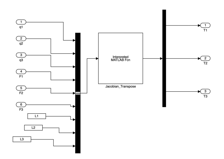
The Jacobian_Transpose function is as follows:

The Jacobian_Transpose function is as follows:
function J_T = Jacobi_T(x)
q1 = x(1);
q2 = x(2);
q3 = x(3);
F1 = x(4);
F2 = x(5);
F3 = x(6);
L1 = x(7);
L2 = x(8);
L3 = x(9);
%%%%%%%%%%%%%%%%%%%%%%%%%%%%%%%%%
J(1,1) = -L1*sin(q1)-L2*sin(q1+q2)-L3/2*sin(q1+q2+q3);
J(1,2) = -L2*sin(q1+q2)-L3/2*sin(q1+q2+q3);
J(1,3) = -L3/2*sin(q1+q2+q3);
J(2,1) = L1*cos(q1)+L2*cos(q1+q2)+L3/2*cos(q1+q2+q3);
J(2,2) = L2*cos(q1+q2)+L3/2*cos(q1+q2+q3);
J(2,3) = L3/2*cos(q1+q2+q3);
J(3,1) = 1;
J(3,2) = 1;
J(3,3) = 1;
F = [F1;F2;F3];
J_T = J'*F;
end

The schematic of the forward kinematics of the 3R robot arm in Simulink is as follows:

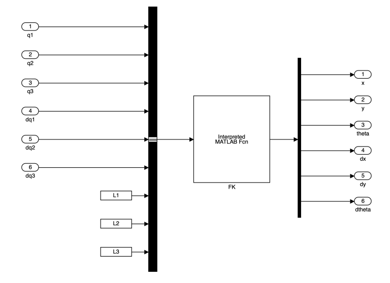
The FK function can be computed using the following code:

function FK = Forward_kinematics(z)
%this function calculated the forward kinematics of the robot
q1 = z(1);
q2 = z(2);
q3 = z(3);
dq1 = z(4);
dq2 = z(5);
dq3 = z(6);
L1 = z(7);
L2 = z(8);
L3 = z(9);
    
X1 = L1*cos(q1)+L2*cos(q1+q2)+L3*cos(q1+q2+q3);
X2 = L1*sin(q1)+L2*sin(q1+q2)+L3*sin(q1+q2+q3);
X3 = q1 + q2 + q3;
X = [X1;X2;X3];
x = [q1;q2;q3;L1;L2;L3];
J = Jacobi(x);
dq = [dq1;dq2;dq3];
dX1 = J(1,1:3)*dq;
dX2 = J(2,1:3)*dq;
dX3 = J(3,1:3)*dq;
dX = [dX1;dX2;dX3];
FK = [X;dX];
end

The main code that you can get the simulation output of the Computed Torque Control (CTC) of the 3R robot arm in task space is as follows:

%the main program
clc
clear
close all
% RRR Parameters
L1 = 2 ;
L2 = 2;
L3 = 2;
m1 = 0.1;
m2 = 0.1;
m3 = 0.1;
W = 0.01;
g = 9.81;
%%%%%%%%%%%%%%%%%%%%%%%%%%%%%%%%%%%%
%Controller
kv = 40;
kp =20;
%%%%%%%%%%%%%%%%%%%%%%%%%%%%%%%%%%%%%%%%
% simulation parameters
T_f = 10; % simulation interval
AT = 1e-6; % absolute tolerance
RT = 1e-6; % relative tolerance
RF = 4; % Refine factor
%%%%%%%%%%%%%%%%%%%%%%%%%%%%%%%%%%%%%%%
% start simulation
q1 = [];
q2 =[];
q3 = [];
dq1 =[];
dq2 = [];
dq3 =[];
x = [];
y = [];
theta = [];
dx = [];
dy = [];
dtheta = [];
F1 = [];
F2 = [];
F3 = [];
sim('RRR_with_CTC_task_space')
%%%%%%%%%%%%%%%%%%%%%%%%%%%%%%%%%%%%%%%
%Plot the links
figure()
for i = 1:5:length(y)
    
    x0 = [0 0];
    x1 = [L1*cos(q1(i)) L1*sin(q1(i))];
    x2 = x1 + [L2*cos(q1(i)+q2(i)) L2*sin(q1(i)+q2(i))];
    x3 = x2 + [L3*cos(q1(i)+q2(i)+q3(i)) L3*sin(q1(i)+q2(i)+q3(i))];
    clf
    plot([x0(1) x1(1)], [x0(2) x1(2)], 'r-');
    hold on
    plot([x1(1) x2(1)], [x1(2) x2(2)], 'g-');
    plot([x2(1) x3(1)], [x2(2) x3(2)], 'b-');
    
    xlim([-4 4])
    ylim([-4 4])
    axis equal
    drawnow 
end
figure
plot(tout,yd,'r')
hold on
plot(tout,y,'b')
legend('yd','y')

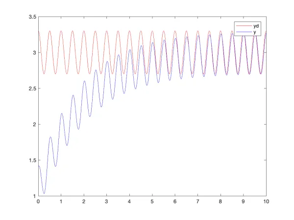
The desired position and orientation are defined to be:

x_{d} = 2.5 y_{d} = 3 + 0.3 c o s (4 π t) θ_{d} = 0

By running this code the following outputs can be achieved:

Output of the Computed Torque Control of a 3R Robot Arm in Task Space

Problem 4.

Objective: Implementing a trajectory and additional simulation of an elastic ball to cause the robot to move to bounce the ball in a stable manner using the results of Problem 3.
Assume you are using a tennis ball, which has a coefficient of restitution of approximately 0.8. In the dynamic modeling of the ball, you can assume that the ball can only move in the vertical direction.

Solution:

Please download the files at the end of this post and look at the “RRR CTC Ball” folder. Note that you should have MATLAB and Simulink installed on your system to be able to run these codes.
Most of the code is pretty much like the previous problem with the addition of the ball simulation.

The main program to run the simulation is as follows:

%the main program
clc
clear
close all
% RRR Parameters
L1 = 2 ;
L2 = 2;
L3 = 2;
m1 = 0.1;
m2 = 0.1;
m3 = 0.1;
W = 0.01;
g = 9.81;
%%%%%%%%%%%%%%%%%%%%%%%%%%%%%%%%%%%%
%Controller
kv = 40;
kp = 20;
%%%%%%%%%%%%%%%%%%%%%%%%%%%%%%%%%%%%%%%%
% simulation parameters
T_f = 5; % simulation interval
AT = 1e-6; % absolute tolerance
RT = 1e-6; % relative tolerance
RF = 4; % Refine factor
%%%%%%%%%%%%%%%%%%%%%%%%%%%%%%%%%%%%%%%
% start simulation
q1 = [];
q2 =[];
q3 = [];
dq1 =[];
dq2 = [];
dq3 =[];
x = [];
y = [];
theta = [];
dx = [];
dy = [];
dtheta = [];
F1 = [];
F2 = [];
F3 = [];
sim('RRR_with_CTC_task_space_ball')
%%%%%%%%%%%%%%%%%%%%%%%%%%%%%%%%%%%%%%%
[t,yball]=BallPosition(y,dy);
%Plot the links
figure()
for i = 1:length(yball)
    
    x0 = [0 0];
    x1 = [L1*cos(q1(i)) L1*sin(q1(i))];
    x2 = x1 + [L2*cos(q1(i)+q2(i)) L2*sin(q1(i)+q2(i))];
    x3 = x2 + [L3*cos(q1(i)+q2(i)+q3(i)) L3*sin(q1(i)+q2(i)+q3(i))];
   
    clf
    
    plot([x0(1) x1(1)], [x0(2) x1(2)], 'r-');
    hold on
    plot([x1(1) x2(1)], [x1(2) x2(2)], 'g-');
    plot([x2(1) x3(1)], [x2(2) x3(2)], 'b-');
    if(~isinf(yball(i)))
        hold on
       plot(xd(i)-0.8,yball(i),'o','LineWidth',4)
    end
    xlim([-1 4])
    ylim([-1 4])
    axis equal
    drawnow 
end
figure
plot(t,yball,'r')
hold on
plot(t,y(1:length(t)))

The “BallPosition” function used above is as follows:

function [t,h]=BallPosition(y,dy)
% initial heigh and velocity of the ball
x0 = [8 -5];
tspan = 0:0.1:10;
[t,x] = ode45(@ball,tspan,x0);
% coefficient of restitution
alpha = 0.8;
h = x(:,1);
v = x(:,2);
t(1) = 0;
dt = 0.01;
g = 9.81;
a = -g;
i = 1;
% 5 is the number of times ball hits the paddle
for n = 1:5
while h(i) > y(i)
    t(i+1) = t(i) + dt;
    v(i+1)=v(i)+a*dt;
    h(i+1)=h(i)+v(i)*dt;
    i=i+1;
end
i = i-1;
v(i) = alpha*(dy(i)-v(i))+dy(i);
end
  
end

The following is the output of the simulation of the 3R robot arm with CTC control playing Ping Pong:

Download all the codes mentioned above HERE.